When the resource analyst lowers the grades above a given cutoff value, there is an underlying assumption that these grades belong to a different population which is distinct from the grades below the cutoff. As the analyst does not know how to deal with the high grades population he treats it in an empirical way, changing the high values.

The important question is why these samples behave in this different way. It must be some reason, detectable or not, as the grade distribution is a result of several physical, and may be chemical, phenomena occurring along the time. A simple example where two different populations can be detected is in a deposit where there is a zone of fractures. In this zone the gold particles will be aggregated to form nuggets. So there is a population of disseminated gold, even in the fractured zone, and a population with high grade samples, looking as there are two different minerals. But it is a very rare case where the reasons of the existence of two populations can be detected.

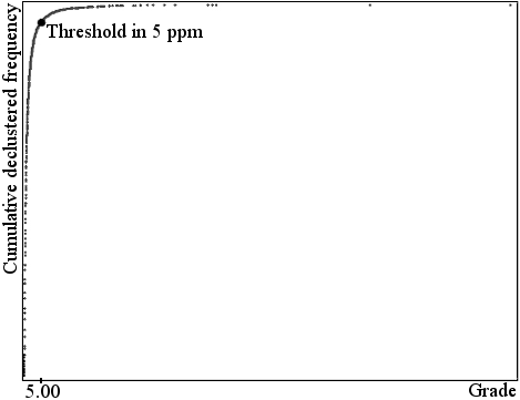
One way to separate the populations is to draw the cumulative frequency of the grade and search for an inflexion point. In Calculus an inflexion point is the point where the first and second derivatives are null. Here this term is used as in the common language: the inflexion point is the point where the angle of the curve with the vertical axis grows significantly. Figure 1 shows the cumulative frequency of gold grades in the Amapari deposit. It can be easily seen that the inflexion point is some value around 5 g/t.

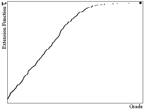
Sometimes there is not a clear inflexion point and FPG treats the whole set of grades as a single population, although the analyst cuts the grades above a chosen value. Figure 2 shows the cumulative frequency of variable V of Walker Lake (Isaaks and Srivastava, 1989) where no inflexion point was found.

But the analysis of the cumulative frequency is not always the best way to separate populations. There are other factors that will not be presented here which can be used for this purpose. The knowledge of the nature of the data and, in the mineral frame, the knowledge of the genesis of the deposit can be very important and sometimes crucial to apply efficiently the techniques of FPG.

Point or derived variables and global or primitive variables
A variable referring to a macroscopic portion associated to a point or derived variable is called a global or a primitive variable. Examples: area, volume or tonnage associated to a grade, or time associated to instantaneous velocity. They are called primitive because they are intuitive and need no definitions: a volume or an area can be seeing, a mass can be touched, and the weight can be felt.
A variable obtained as a ratio of two primitive variables, measured in a portion that can be considered as a point is called a point variable or a derived variable. Examples: instantaneous velocity in m/sec, a sample grade in %, g/t among others.

Absolute natural classes and conditional natural classes
In FPG theory N(d) = (tmax– tmin) / d  is called the number of absolute natural classes associated to the precision d, where tmax and tmin are respectively the maximum and minimum grade values taking into account the possible extreme values. Consequently, the number of natural classes is the same as the possible values.
A conditional natural class is the interval between two sequential measured values. The number of conditional natural classes is the same as the number of different measured values. It is conditioned to the set of values of the samples.

Redefinition of the concept of average
In FPG theory the average is divided into several types:

Ordinary Kriging weights
As in FPG theory an ordinary kriging weight represents a probability or an extension, the weight can never be negative. Sometimes mathematical results have no physical meaning. A theorem provides the best correction to negative weights (Armony, 2000).
It must be also understood that kriging weights are associated to the axiom of continuity and have nothing to do with representativeness.