FPG Theory

Following the previous analysis, a consistent theory was built, based on a variable transformation that was called Field Parametric Geostatistics (FPG). The principal aim of FPG was to build a variable that fulfils all the conditions pointed out above.
The mathematical formulation is shown in another section, but the procedure is easy to understand:
- Assign to each sample a declustering weight. If there is not a declustering procedure, the weight is one. Declustering can be obtained with declus from GSLIB (Deutsch and Journel, 1998).
- Sum up all the declustering weights of the same grade – the result is the extension of the grade.
- Build the cumulative extension of the grades – it is self explanatory.
Standardised cumulative extension of the grades – the cumulative extension of the grades is standardized to range from zero to one.
When dealing with tonnages as extensions and the density is not constant, the declustering weight must be multiplied by the density.
Standardised cumulative extension of the grades is the new chosen variable. It carries both the grade and the extension values, because it refers to extensions of the grades and is isomorphic to the grades set. It fulfils the needs required for the variable to be modelled: uses all the available information, obeys both axioms and is a discrete variable.
Standardised cumulative extension is called the extension function. It is a totally discrete function because it has a finite number of points.
The extension function is not:
- A simple uniform transform.
- A probability function.
- A distribution function.
An extension represents a real physical entity, not only a kind of modified frequency.
The mathematical symbol of the variable is the Greek letter τ.
The usage of the new variable (τ = standardized cumulative extension of the grade):
- Transforms bad or noisy variograms into well-behaved variograms as it can be seen in Figures 1 and 2 where variograms of the synthetic 140 points presented in GSLIB are shown. When the distribution is symmetric or almost symmetric, the variograms have the same shape, as shown at Figures 3 and 4. Moreover, in the last case kriging results are similar.
- Reduces automatically the influence of the high grades without manual intervention.
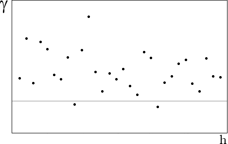
Fig. 1
Variogram shape of the 140 samples of GSLIB synthetic data.
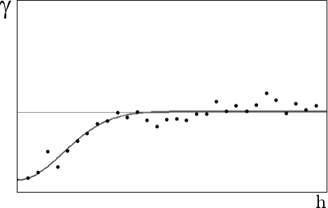
Fig. 2
Variogram shape of the FPG transform of the 140 GSLIB synthetic data.
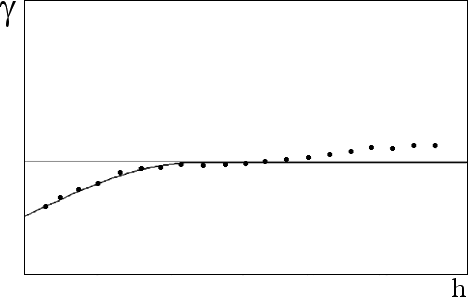
Fig. 3
Variogram shape of the thickness of a kaolin layer in the Amazon state, Brazil.
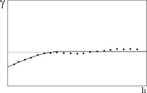
Fig. 4
Variogram shape of the FPG transform of thickness of the same kaolin layer.
In a small squared mining unit four blast holes are drilled in an almost symmetric way as shown in Figure 1.
The assayed samples have as results the grades 1.00 g/t, 2.00 g/t, 3.00 g/t and 90.00 g/t of gold. The precision of the grades is two decimals. Figure 2 shows an extension function conditioned to the four values. Note that although the lines segments seem to be continuous they are sequences of points associated with the given precision. From 1.00 g/t to 2.00 g/t there are 100 points. From 2.00 g/t to 3.00 g/t there are 100 points. From 3.00 g/t to 90.00 g/t there are 8 700 points.
As the holes are inside a small block it can be assumed that all the points of the block are associated to a unique random variable and the extension function can be treated as a probability function, a conditional cumulative distribution function (ccdf). The probability to obtain a new sample with grade between 1.00 g/t and 2.00 g/t, between 2.00 g/t and 3.00 g/t, and between 3.00 g/t and 90.00 g/t has the same value 0.25. But the probability to get a new sample with exactly 90.00 g/t is 87 times lower than to get a sample with grade 3.00 g/t, for example.
In the continuous spectrum this conclusion would be very difficult to reach.
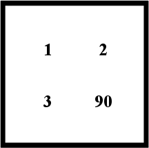
Fig. 1
A squared mining unit with four blast holes.
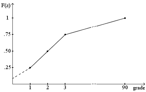
Fig. 2
CCDF of the grades inside the mining unit.
Procedure guidelines for mineral resources estimation assuming a single population:
- Data analysis;
- Declustering, if necessary. If not, assign the unity as the declustering weight for all the samples;
- FPG transform: create a piecewise linear extension function;
- Variography of the transformed variable;
- Kriging the transformed variable;
- Back-transformthe results to grades by linear interpolation in the extension function.
Procedure guidelines for mineral resources estimation assuming two populations:
- Data analysis.
- Assign carefully the inflexion point (see the section “The inflexion point”);
- Lower grades: use Classical Geostatistics;
- Higher grades: use FPG transform;
- For both low and high grades: variography and kriging;
- Back-transform for FPG results;
- Indicator variogram and indicator kriging;
- The final grade of each block is obtained by weighting, using the proportions given by indicator kriging.
